# Select organisms that should be included in the analysis
otu_table_tax <- subset_taxa(otu_ctrl_clean, kingdom == "Bacteria")
# Remove organisms that should not be included in the analysis
otu_table_tax <- subset_taxa(otu_table_tax, order != "Chloroplast" &
family != "Mitochondria")
# Count OTUs before and after filtering
ntaxa(otu_ctrl_clean) # 25390
ntaxa(otu_table_tax) # 22046 (~13% of the OTUs were filtered out)Global filtering
A global filtering is typically applied early to preserve only relevant taxonomic assignations and remove very low-count OTUs that are disproportionately driven by sequencing/PCR error and index misassignment, thereby reducing noise and improving downstream compositional and multivariate analyses.
This section documents how to filter OTUs based on taxonomic assignations and filter out singletons and rare OTUs based on absolute or relative abundance thresholds in phyloseq objects. To follow the example presented on this page directly on your computer, download the script 004_global_filter.R and the example raw data by clicking the buttons below. Alternatively, you may copy the codes below into your own script, and use your own data.
Taxonomy filtering
This first simple step serves to preserve only the relevant OTUs that were targeted with each primer sets: i.e., Bacteria for 16S, Fungi for ITS and Metazoa for CO1.
Note that the 16S primers amplifying the V4-V5 regions are also suitable for Archaea. The choice to include them or not in the following filtering depends on the hypotheses of your study. Similarly, primers targeting the internal transcribed spacer (ITS1 and ITS2) regions, while commonly used as the universal barcoding marker for fungi, often co-amplify DNA from a wide variety of other Eukaryotes due to the conserved nature of the flanking ribosomal RNA genes (18S, 5.8S, and 28S). For example, DNA from plants and protists is often amplified using these primers. It is recommended to filter them out when the hypotheses of the study are focused on Fungi. Finally, CO1 primers may also amplify Prokaryotes or other Eukaryotes, but these are not specificly targeted and should be filtered out.
| Name | Target | Primers (sequence 5’-3’) | Regions | Length | References |
|---|---|---|---|---|---|
| 16S | Prokaryotes (Bacteria and Archaea) | 515F-Y (GTGYCAGCMGCCGCGGTAA) 926RB (CCGYCAATTYMTTTRAGTTT) |
V4-V5 | 360-500 bp (~460 bp) |
[1] |
| ITS | Fungi | ITS9MUN (TGTACACACCGCCCGTCG) ITS4ngsUni (CCTSCSCTTANTDATATGC) |
ITS1-ITS2 | 150-1200 bp (~280 bp) |
[2] |
| CO1 | Metazoa | mlCOIintF (GGWACWGGWTGAACWGTWTAYCCYCC) jgHCO2198 (TAIACYTCIGGRTGICCRAARAAYCA) |
320-345 658 |
250-700 (~313 bp) |
[3,4] |
This demonstration is done with the 16S data, and we choose to keep only Bacteria. Additional organisms may have been amplified using the above-mentioned primers. For example, Chloroplast and Mitochondria have a 16S gene because they are ancestral bacteria. However, they come from plant or animal tissue and should therefore be removed.
In this demonstration, ~2% of OTUs were not Bacteria, and ~11% were either Chloroplast or Mitochondria.
Which organisms to preserve or to remove from your data set depends on your sample type (e.g., soil vs water) and the origin of your sample (e.g., tropical vs arctic). In this demonstration, we have soil samples from a European temperate forest that have a high chance of containing plant material, thus we know that a large amount of Chloroplast and Mitochondria is expected. Similarly, when looking at the CO1 gene, depending on our research aim, it may be relevant to remove anything that is not expected in a data set of European temperate forest soil samples (e.g., Gorilla and Starfish).
Singletons and rare OTUs
Singletons and other rare OTUs are predominantly composed of PCR, sequencing, and chimera artefacts, and their removal has been shown to have negligible effects on hypothesis-driven community comparisons while substantially reducing noise[5–8]. Retaining them is mainly justified in studies explicitly targeting rare biosphere diversity and requires careful validation[9]. Consequently, filtering rare features simplifies microbiome data sets without materially altering ecological inference in most comparative analyses.
In R, singletons are typically removed by excluding OTUs with a total count of one across all samples, while rare OTUs are filtered by applying absolute (e.g. total counts <5 or <10) or relative abundance thresholds (e.g. <0.01%) to the OTU table[5,6,9], commonly using phyloseq::prune_taxa() in combination with taxa_sums().
Removing singletons
Removing singletons is as simple as keeping anything that has more than 1 read throughout the entire data set.
# Remove singletons
otu_table_single <- prune_taxa(taxa_sums(otu_table_tax) > 1, otu_table_tax)
# Count OTUs after filtering
ntaxa(otu_table_single) # 21632 (~2% of the remaining OTUs were singletons)Removing rare OTUs
OTUs are considered rare if their abundance is small compared to other OTUs. They may be present in many samples, but if their total sum across samples is smaller than k% of the average sequencing depth (relative abundance), or smaller than k reads (absolute abundance) then they are considered rare.
NOTE: When calculating the average sequencing depth, ignore controls and blanks, as they artificially lower the average.
Relative abundance
Typically, thresholds between 0.005% and 0.1% relative abundance are found in the literature. For the sake of this demonstration, we’ve included multiple thresholds between 0.005% and 0.1%, as well as a threshold up to 1% to better illustrate the effects of filtering out rare OTUs on different community analyses.
We define relative thresholds based on the average sequencing depth (assuming that all samples have sufficient sequencing depth).
# Calculate the average sequencing depth
seq_depth_avg <- mean(sample_sums(otu_table_tax)) # 139853.2 reads
# Calculate thresholds based on k% of the average sequencing depth
# For the sake of this exercise, multiple thresholds between 0.005% and 1% are
# tested to compare their effects on various community analyses.
thresh005 <- ceiling(seq_depth_avg*0.005/100) # 7 reads
thresh01 <- ceiling(seq_depth_avg*0.01/100) # 14 reads
thresh05 <- ceiling(seq_depth_avg*0.05/100) # 70 reads
thresh1 <- ceiling(seq_depth_avg*0.1/100) # 140 reads
thresh10 <- ceiling(seq_depth_avg*1/100) # 1399 reads
# Remove all OTUs that have a total sum lower than the threshold
otu_table_rare005 <- otu_table_tax %>% prune_taxa(taxa_sums(.) > thresh005, .)
otu_table_rare01 <- otu_table_tax %>% prune_taxa(taxa_sums(.) > thresh01, .)
otu_table_rare05 <- otu_table_tax %>% prune_taxa(taxa_sums(.) > thresh05, .)
otu_table_rare1 <- otu_table_tax %>% prune_taxa(taxa_sums(.) > thresh1, .)
otu_table_rare10 <- otu_table_tax %>% prune_taxa(taxa_sums(.) > thresh10, .)
# Compare the number of OTU in each filtering step
ntaxa(otu_ctrl_clean) #25390 (before filtering)
ntaxa(otu_table_tax) #22046 (~87% of OTUs are Bacteria)
ntaxa(otu_table_single) #21632 (~2% singletons)
ntaxa(otu_table_rare005) #8064 (~63% of OTUs have less than 7 reads; 0.005%)
ntaxa(otu_table_rare01) #6183 (~72% of OTUs have less than 14 reads; 0.01%)
ntaxa(otu_table_rare05) #3467 (~84% of OTUs have less than 70 reads; 0.05%)
ntaxa(otu_table_rare1) #2710 (~88% of OTUs have less than 140 reads; 0.1%)
ntaxa(otu_table_rare10) #979 (~96% of OTUs have less than 1399 reads; 1%)Absolute abundance
Typically, thresholds between 5-10 reads are found in the literature. In this example, this roughly corresponds to a relative abundance threshold at 0.005% (8 reads). If the average sequencing depth of your data set is larger than the one presented here, it may be relevant to test removing 5 and 10 reads if those absolute thresholds are significantly lower than a relative threshold at 0.005%.
Compare thresholds
To visualize the effect of these different thresholds, we must first create a data frame per filtered OTU table that summarizes the sequencing depth per sample and the Observed OTU (richness).
# Non-filtered OTU table
seq_depth_raw <- cbind.data.frame(sample_data(otu_table_tax)) %>%
cbind(estimate_richness(otu_table_tax, measures = "Observed")) %>%
mutate(LibrarySize = sample_sums(otu_table_tax)) %>%
arrange(LibrarySize) %>% mutate(Index = row_number()) %>%
mutate(seq_depth = "raw")
# Singletons
seq_depth_single <- cbind.data.frame(sample_data(otu_table_single)) %>%
cbind(estimate_richness(otu_table_single, measures = "Observed")) %>%
mutate(LibrarySize = sample_sums(otu_table_single)) %>%
arrange(LibrarySize) %>% mutate(Index = row_number()) %>%
mutate(seq_depth = "singletons")
# Rare 0.005% (<7 reads)
seq_depth_rare005 <- cbind.data.frame(sample_data(otu_table_rare005)) %>%
cbind(estimate_richness(otu_table_rare005, measures = "Observed")) %>%
mutate(LibrarySize = sample_sums(otu_table_rare005)) %>%
arrange(LibrarySize) %>% mutate(Index = row_number()) %>%
mutate(seq_depth = "rare 0.005%")
# Rare 0.01% (<14 reads)
seq_depth_rare01 <- cbind.data.frame(sample_data(otu_table_rare01)) %>%
cbind(estimate_richness(otu_table_rare01, measures = "Observed")) %>%
mutate(LibrarySize = sample_sums(otu_table_rare01)) %>%
arrange(LibrarySize) %>% mutate(Index = row_number()) %>%
mutate(seq_depth = "rare 0.01%")
# Rare 0.05% (<70 reads)
seq_depth_rare05 <- cbind.data.frame(sample_data(otu_table_rare05)) %>%
cbind(estimate_richness(otu_table_rare05, measures = "Observed")) %>%
mutate(LibrarySize = sample_sums(otu_table_rare05)) %>%
arrange(LibrarySize) %>% mutate(Index = row_number()) %>%
mutate(seq_depth = "rare 0.05%")
# Rare 0.1% (<140 reads)
seq_depth_rare1 <- cbind.data.frame(sample_data(otu_table_rare1)) %>%
cbind(estimate_richness(otu_table_rare1, measures = "Observed")) %>%
mutate(LibrarySize = sample_sums(otu_table_rare1)) %>%
arrange(LibrarySize) %>% mutate(Index = row_number()) %>%
mutate(seq_depth = "rare 0.1%")
# Rare 1% (<1399 reads)
seq_depth_rare10 <- cbind.data.frame(sample_data(otu_table_rare10)) %>%
cbind(estimate_richness(otu_table_rare10, measures = "Observed")) %>%
mutate(LibrarySize = sample_sums(otu_table_rare10)) %>%
arrange(LibrarySize) %>% mutate(Index = row_number()) %>%
mutate(seq_depth = "rare 1%")
# Combine data frames
seq_depth_all <- seq_depth_raw %>% rbind(seq_depth_single) %>%
rbind(seq_depth_rare005) %>% rbind(seq_depth_rare01) %>%
rbind(seq_depth_rare05) %>% rbind(seq_depth_rare1) %>%
rbind(seq_depth_rare10)Effect on library size
# Plot the library size of all samples
ggplot(data = seq_depth_all, aes(x = Index, y = LibrarySize, color = seq_depth)) +
geom_point() + geom_line()With this analysis, we can see that the first filtering step (singletons) does not affect LibrarySize, as the points completely overlap (yellow vs brown). Aside from a threshold at 1%, other thresholds barely reduced library size per sample.
Tip
Try zooming in on a selection of points with low library size or large library size to better see the effects of the different thresholds. For example, the filtering of rare OTUs at a threshold of 0.01% changes very little in the LibrarySize, even though we lost ~72% of OTUs.
Effect on OTU richness
To confirm our choice of the best filtering threshold, let’s compare the effect of filtering on OTU richness.
# Plot the OTU richness of all samples
ggplot(data = seq_depth_all, aes(x = Index, y = Observed, color = seq_depth)) +
geom_point() + geom_line()This plot shows that these different filtering thresholds return the same pattern of OTU richness as a function of library size.
Tip
Try comparing other alpha diversity indices, such as the Shannon index.
# Add Shannon index to each OTU table as such
seq_depth_raw <- seq_depth_raw %>%
cbind(estimate_richness(otu_table_tax, measures = "Shannon"))
# Plot the Shannon index of all samples
ggplot(data = seq_depth_all, aes(x = Index, y = Shannon, color = seq_depth)) +
geom_point() + geom_line()Filtering rare OTUs has no significant effect on the Shannon index. Note also the lack of a clear relationship between the Shannon index and LibrarySize.
Effect on beta diversity
To confirm our choice of filtering further, we can compare how the different filtering methods affect beta diversity.
# Non-filtered OTU table
beta_div_raw <- otu_table_tax %>%
tax_transform("identity", rank = "taxa_OTU") %>%
dist_calc("aitchison") %>%
ord_calc("PCoA") %>%
ord_plot(color = "Land_use", auto_caption = NA) +
stat_ellipse(aes(colour = Land_use))
# Singletons
beta_div_single <- otu_table_single %>%
tax_transform("identity", rank = "taxa_OTU") %>%
dist_calc("aitchison") %>%
ord_calc("PCoA") %>%
ord_plot(color = "Land_use", auto_caption = NA) +
stat_ellipse(aes(colour = Land_use))
# Rare 0.005%
beta_div_rare005 <- otu_table_rare005 %>%
tax_transform("identity", rank = "taxa_OTU") %>%
dist_calc("aitchison") %>%
ord_calc("PCoA") %>%
ord_plot(color = "Land_use", auto_caption = NA) +
stat_ellipse(aes(colour = Land_use))
# Rare 0.01%
beta_div_rare01 <- otu_table_rare01 %>%
tax_transform("identity", rank = "taxa_OTU") %>%
dist_calc("aitchison") %>%
ord_calc("PCoA") %>%
ord_plot(color = "Land_use", auto_caption = NA) +
stat_ellipse(aes(colour = Land_use))
# Rare 0.05%
beta_div_rare05 <- otu_table_rare05 %>%
tax_transform("identity", rank = "taxa_OTU") %>%
dist_calc("aitchison") %>%
ord_calc("PCoA") %>%
ord_plot(color = "Land_use", auto_caption = NA) +
stat_ellipse(aes(colour = Land_use))
# Rare 0.1%
beta_div_rare1 <- otu_table_rare1 %>%
tax_transform("identity", rank = "taxa_OTU") %>%
dist_calc("aitchison") %>%
ord_calc("PCoA") %>%
ord_plot(color = "Land_use", auto_caption = NA) +
stat_ellipse(aes(colour = Land_use))
# Rare 1%
beta_div_rare10 <- otu_table_rare10 %>%
tax_transform("identity", rank = "taxa_OTU") %>%
dist_calc("aitchison") %>%
ord_calc("PCoA") %>%
ord_plot(color = "Land_use", auto_caption = NA) +
stat_ellipse(aes(colour = Land_use))
# Visualize all plots together
ggarrange(beta_div_raw, beta_div_single, beta_div_rare005, beta_div_rare01,
beta_div_rare05, beta_div_rare1, beta_div_rare10,
labels = c(
"Non-filtered (22046 OTUs)", "Singletons (21632 OTUs)",
"0.005% (<7 reads; 8064 OTUs)", "0.01% (<14 reads; 6183 OTUs)",
"0.05% (<70 reads; 3467 OTUs)", "0.1% (<140 reads; 2710 OTUs)",
"1% (<1399 reads; 979 OTUs)"),
ncol = 3, nrow = 3, common.legend = TRUE,
hjust = 0, label.x = 0.2, font.label = list(size = 10))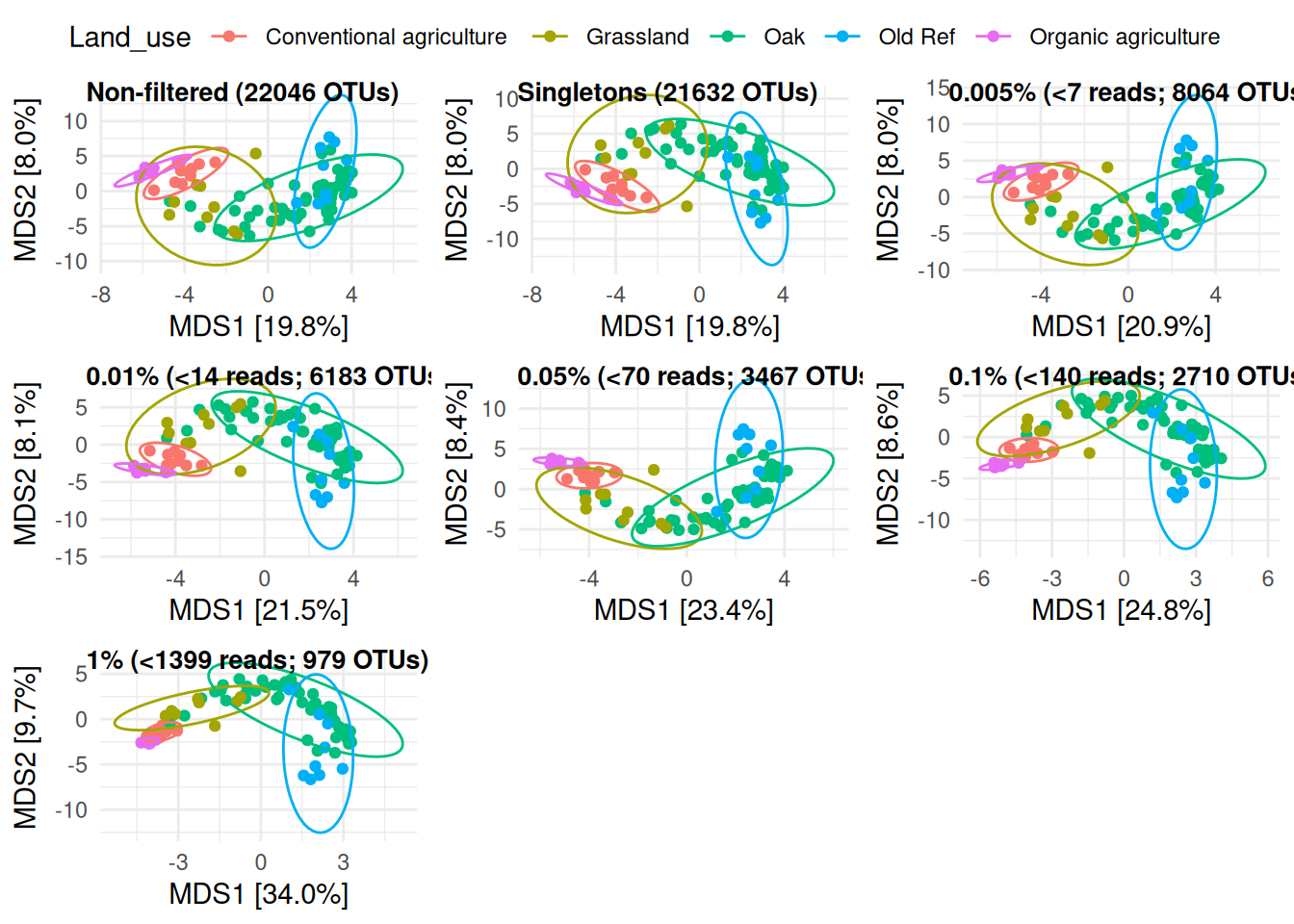
With this analysis, we can see that removing rare OTUs reduces the variance within treatment a little bit, but does not affect overall patterns. Overall, all three plots showed that rare OTUs were mostly found in samples with large library size, and filtering out rare OTUs does not affect patterns. Only a threshold as high as 1% considerably affected patterns.
Choosing the best threshold
Ultimately, the choice of the “best” threshold is completely arbitrary. Various thresholds are found in the literature and no one is more justified than another. As a reminder: singletons and other rare OTUs have been previously found to be predominantly composed of artefacts, thus, their removal has been shown to have negligible effects on hypothesis-driven community comparisons while substantially reducing noise[5–8]. Retaining them is only justified in studies explicitly targeting rare biosphere diversity and requires careful validation[9].
As seen in this demonstration, all thresholds below 1% had little observable effect on library size, alpha diversity and beta diversity. For the sake of being more conservative, let’s select the lowest relative abundance threshold (0.005%), which also roughly corresponded to a conservative absolute threshold (5-10 reads).
# Select the best filtering threshold (0.005%)
# ~63% of OTUs have less than 7 reads
otu_table_rare <- otu_table_rare005Clean and save OTU table
# OTU table with singletons filtered
save(otu_table_single, file = "RData/16S/otu_single_clean.RData")
# OTU table with rare taxa filtered
save(otu_table_rare, file = "RData/16S/otu_rare_clean.RData")References
1. Parada, A. E., Needham, D. M., & Fuhrman, J. A. (2015). Every base matters: assessing small subunit rRNA primers for marine microbiomes with mock communities, time series and global field samples. Environmental Microbiology, 18(5), 1403–1414. https://doi.org/10.1111/1462-2920.13023
2. Tedersoo, L., & Lindahl, B. (2016). Fungal identification biases in microbiome projects. Environmental Microbiology Reports, 8(5), 774–779. https://doi.org/10.1111/1758-2229.12438
3. Leray, M., Yang, J. Y., Meyer, C. P., Mills, S. C., Agudelo, N., Ranwez, V., Boehm, J. T., & Machida, R. J. (2013). A new versatile primer set targeting a short fragment of the mitochondrial COI region for metabarcoding metazoan diversity: application for characterizing coral reef fish gut contents. Frontiers in Zoology, 10(1), 34. https://doi.org/10.1186/1742-9994-10-34
4. Geller, J., Meyer, C., Parker, M., & Hawk, H. (2013). Redesign of PCR primers for mitochondrial cytochrome c oxidase subunit I for marine invertebrates and application in all-taxa biotic surveys. Molecular Ecology Resources, 13(5), 851–861. https://doi.org/10.1111/1755-0998.12138
5. Edgar, R. C. (2016). UNOISE2: Improved error-correction for illumina 16S and ITS amplicon sequencing. http://dx.doi.org/10.1101/081257
6. Nikodemova, M., Holzhausen, E. A., Deblois, C. L., Barnet, J. H., Peppard, P. E., Suen, G., & Malecki, K. M. (2023). The effect of low-abundance OTU filtering methods on the reliability and variability of microbial composition assessed by 16S rRNA amplicon sequencing. Frontiers in Cellular and Infection Microbiology, 13. https://doi.org/10.3389/fcimb.2023.1165295
7. Sgarbi, L. F., Bini, L. M., Heino, J., Jyrkänkallio-Mikkola, J., Landeiro, V. L., Santos, E. P., Schneck, F., Siqueira, T., Soininen, J., Tolonen, K. T., & Melo, A. S. (2020). Sampling effort and information quality provided by rare and common species in estimating assemblage structure. Ecological Indicators, 110, 105937. https://doi.org/10.1016/j.ecolind.2019.105937
8. Cao, Y., Wu, G., & Yu, D. (2021). Include macrofungi in biodiversity targets. Science, 372(6547), 1160–1160. https://doi.org/10.1126/science.abj5479
9. Brown, S. P., Veach, A. M., Rigdon-Huss, A. R., Grond, K., Lickteig, S. K., Lothamer, K., Oliver, A. K., & Jumpponen, A. (2015). Scraping the bottom of the barrel: are rare high throughput sequences artifacts? Fungal Ecology, 13, 221–225. https://doi.org/10.1016/j.funeco.2014.08.006