Dealing with positive controls

This section documents how to inspect positive controls to confirm successful amplification of target genes, detect false results, and overall, verify that the full workflow (from extraction to bioinformatics) behaves as expected^[1].

To follow the example presented on this page directly on your computer, download the script 003_positive_control.R and the example raw data by clicking the buttons below. Alternatively, you may copy the codes below into your own script, and use your own data.

Inspect samples

Positive controls added before sequencing usually contain a synthetic community (OTUs absent from true samples) and serve to demonstrate successful amplification of target genes or provide information about tag-switching.

# Load raw OTU table
load("RData/16S/otu_table_raw.RData")

To inspect this data set, convert OTU table from count data to both a presence-absence table and a relative abundance table.

# Convert OTU table from count data to presence-absence
otu_table.pa <- transform_sample_counts(otu_table_raw, function(x) 1*(x>0))

# Convert OTU table from count data to relative abundance
otu_table.rel <- transform_sample_counts(otu_table_raw, function(x) x/sum(x))

Identify synthetic community

# Identify OTUs present in positive controls
otu_table.pa.pos <- prune_samples(
  sample_data(otu_table.pa)$sample_type == "positive control", otu_table.pa)

table.pa.pos <- data.frame(pa.pos = taxa_sums(otu_table.pa.pos))

otu_pos <- filter(table.pa.pos, pa.pos > 0) %>% rownames()

# Filter OTU table to keep only OTUs found in positive controls
otu_table_pos <- prune_taxa(otu_pos, otu_table.rel)

# Visualize the abundance of these OTUs in all samples
plot_bar(otu_table_pos, fill = "kingdom") + 
  facet_grid(~sample_type, scales = "free", space = "free")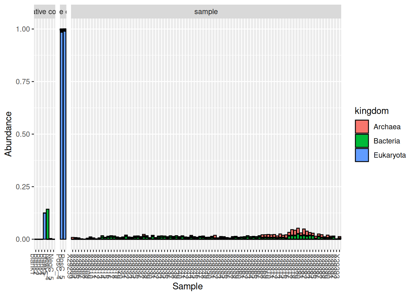

As can be seen on this graph, the synthetic community added to these samples was composed of Eukaryota, but some additional contaminants (probably from true samples) can also be found in the positive controls. The issue of contaminants can be dealt with using the R package decontam as demonstrated in the previous section: Dealing with negative controls.

The rest of the synthetic community will be automatically removed from our data sets while performing taxonomic filtering.

Compare community profiles

If one suspects issues with library preparation or sequencing, positive controls can be used for visual inspection, by making sure the taxonomic profiles match expectations.

# Keep only positive controls for visualization
otu_table.rel.pos <- prune_samples(
  sample_data(otu_table.rel)$sample_type == "positive control", otu_table.rel)

# Visualize the community profiles of these samples
plot_bar(otu_table.rel.pos, fill = "kingdom")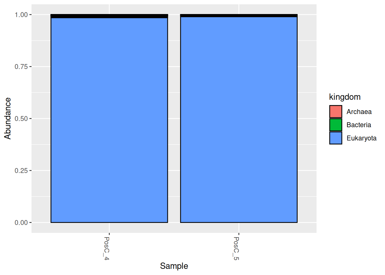

Clean and save OTU table

remove_taxa

Homemade function remove_taxa: a simplified way of removing a selection of OTU from a phyloseq object.

remove_taxa <- function(badTaxa, physeq){
  allTaxa <- taxa_names(physeq)
  cleanTaxa <- allTaxa[!(allTaxa %in% badTaxa)]
  return(prune_taxa(cleanTaxa, physeq))
}

# Remove positive controls
otu_ctrl_pos_clean <- prune_samples(
  sample_data(otu_table_raw)$sample_type != "positive control", otu_table_raw)

# Save cleaned OTU table
save(otu_ctrl_pos_clean, file = "RData/16S/otu_ctrl_pos_clean.RData")

References

1. Lear, G., Dickie, I., Banks, J., Boyer, S., Buckley, H., Buckley, T., Cruickshank, R., Dopheide, A., Handley, K., Hermans, S., Kamke, J., Lee, C., MacDiarmid, R., Morales, S., Orlovich, D., Smissen, R., Wood, J., & Holdaway, R. (2018). Methods for the extraction, storage, amplification and sequencing of DNA from environmental samples. New Zealand Journal of Ecology. https://doi.org/10.20417/nzjecol.42.9