Dealing with negative controls

This section documents how to inspect negative controls (or blanks) and remove contaminant DNA sequences using the R package decontam^[1].

To follow the example presented on this page directly on your computer, download the script 003_negative_control.R and the example raw data by clicking the buttons below. Alternatively, you may copy the codes below into your own script, and use your own data.

Inspect samples

Before using the package decontam to remove contaminants, we must first inspect samples (and controls) to determine if there are any visible problems. We can do this by comparing library size between samples, visualizing the prevalence of OTUs in samples and controls and visualizing the relative abundance of potential contaminants in all samples.

# Load OTU table
load("RData/16S/otu_table_raw.RData")

Library size

The library size (a.k.a. the sequencing depth) of each sample can be predicted based on the type of samples you work with. For example, with soil samples, we expect abundant microbial communities, with hundreds if not thousands of sequences per sample. On the other hand, negative controls and blanks should have very small library sizes.

# Summarize sequencing depth per sample
seq_depth <- cbind.data.frame(sample_data(otu_table_raw)) %>%
  mutate(LibrarySize = sample_sums(otu_table_raw)) %>%
  # Sort the data set by LirarySize and create an Index to match the sorted data
  arrange(LibrarySize) %>% mutate(Index = row_number())

# Visualize LibrarySize as a function of Index, 
# to compare library size between samples
ggplot(data = seq_depth, aes(x = Index, y = LibrarySize, color = sample_type)) +
  geom_point()

We can see that, compared to the rest of the samples, all controls have a small library size. Nevertheless, if you zoom in on the negative controls, you can see that all negative controls have a library size larger than zero. Therefore, further analyses are required to know if the OTUs present in negative controls are contaminants.

Note that positive controls have a larger library size than the negative controls, showing that sequencing performed well in these samples. This can be further confirmed in the previous section: Dealing with positive controls.

Furthermore, one sample has a very small library size compared to other samples (and compared to controls). This sample should be further inspected to determine if its microbial community resemble that of other samples (i.e., replicates). If not, further investigation would be required to determine why this sample is different from other replicates: was there a methodological issue with this sample that resulted in the low sequencing depth; or is this a true biological exception that can occur among your replicates? When in doubt, ask those who collected and processed the samples.

Inspect sample with small library size

# Identify sample with a small library size
subset(seq_depth, sample_type == "sample" & LibrarySize < 10000)

The sample X29239 was taken on the site Oak_51.

  SiteID    PlotID Year_planted Age Soil_ID sample_type
1 Oak_51 Oak_51_NE         1970  51  X29327      sample
2 Oak_51 Oak_51_NW         1970  51  X29328      sample
3 Oak_51 Oak_51_SE         1970  51  X29329      sample
4 Oak_51 Oak_51_SW         1970  51  X29330      sample
5 Oak_51  Oak_51_B         1970  51  X29239      sample

To compare these samples: first, add a column to the sample data in the phyloseq object to identify this sample; then, visualize the samples in an ordination.

# Add a column to sample data in phyloseq object to identify this sample
sample_data(otu_table_raw)$low_depth <- sample_data(otu_table_raw)$Soil_ID=="X29239"

# Plot an ordination of all samples to compare the low seq sample to replicates
otu_table_raw %>%
  tax_transform("identity", rank = "taxa_OTU") %>%
  dist_calc("aitchison") %>%
  ord_calc("PCoA") %>%
  ord_plot(color = "SiteID", shape = "low_depth", auto_caption = NA) +
  stat_ellipse(aes(colour = SiteID))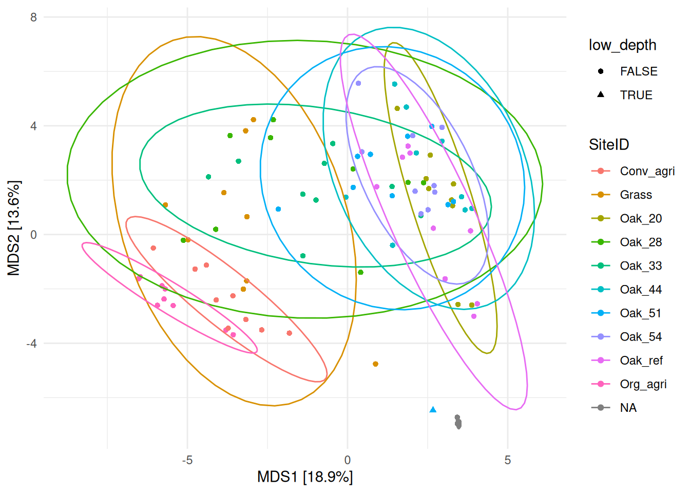

The sample X29239 (shown with a triangle) is located far away from samples of the same site (Oak_51, in light blue), and close to the controls (NA, in gray) demonstrating that it harbors a different community composition than samples from the same site. If this difference cannot be explained, this sample should be removed.

Prevalence of OTUs in negative controls

# For the following analyses, remove positive controls from the data set
otu_table_raw.noPos <- prune_samples(
  sample_data(otu_table_raw)$sample_type != "positive control", otu_table_raw)

First, visualize the prevalence of OTUs in samples and controls:

# Make phyloseq objects of presence-absence in controls and true samples
otu_table.pa <- transform_sample_counts(otu_table_raw.noPos, function(x) 1*(x>0))
otu_table.pa.neg <- prune_samples(
  sample_data(otu_table.pa)$sample_type == "negative control", otu_table.pa)
otu_table.pa.sam <- prune_samples(
  sample_data(otu_table.pa)$sample_type == "sample", otu_table.pa)

# Make data.frame of prevalence in controls and true samples
otu_table.pa <- data.frame(pa.sam = taxa_sums(otu_table.pa.sam),
                           pa.neg = taxa_sums(otu_table.pa.neg))

# Plot the prevalence of OTU in negative controls vs true samples
ggplot(data=otu_table.pa, aes(x=pa.neg, y=pa.sam)) + geom_point() +
  xlab("Prevalence (Negative Controls)") + ylab("Prevalence (True Samples)")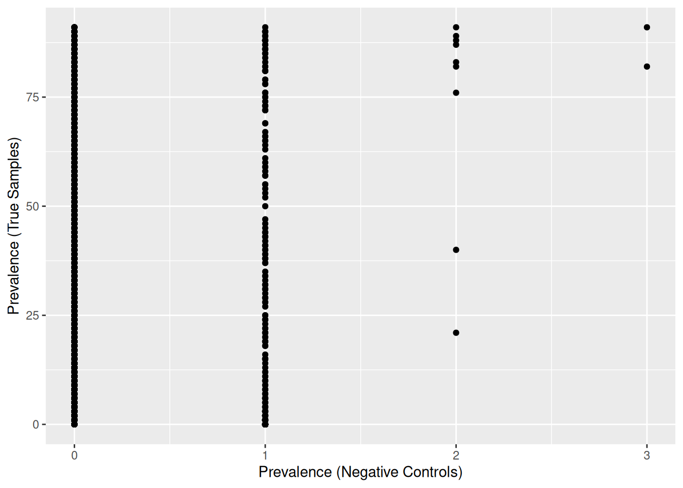

302 OTUs were found in negative controls, and many of them are present in at least one negative control (‘Prevalence (Negative Controls)’ >= 1).

We must find out if there was a contamination in our samples from the method, or if the negative samples have been contaminated by the other samples.

# For further analyses, convert OTU table from count data to relative abundance
otu_table_rel <- transform_sample_counts(otu_table_raw.noPos, function(x) x/sum(x))

# Identify OTUs present in negative controls
otu_neg <- filter(otu_table.pa, pa.neg > 0) %>% rownames()

# Filter OTU table to keep only OTUs found in negative controls
otu_table_neg <- prune_taxa(otu_neg, otu_table_rel)

# Visualize the abundance of these OTUs in all samples
plot_bar(otu_table_neg, fill = "phylum") +
  facet_grid(~sample_type, scales = "free", space = "free")

Warning: `aes_string()` was deprecated in ggplot2 3.0.0.
ℹ Please use tidy evaluation idioms with `aes()`.
ℹ See also `vignette("ggplot2-in-packages")` for more information.
ℹ The deprecated feature was likely used in the phyloseq package.
  Please report the issue at <https://github.com/joey711/phyloseq/issues>.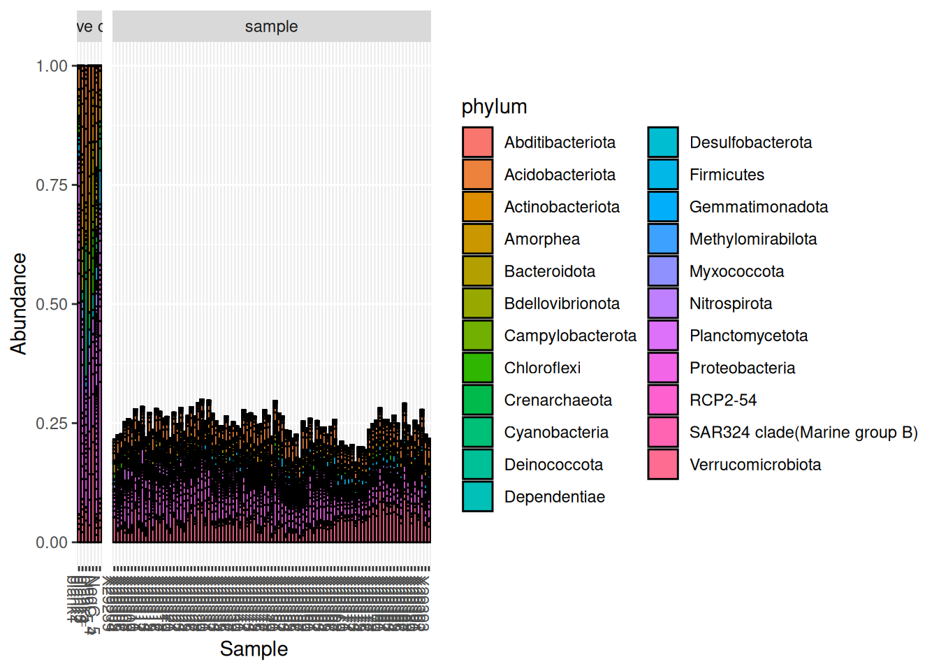

A commonly recommended practice with negative controls is to remove any OTU found in negative controls from the rest of the data set^[2]. However, as you can see in this demonstration, the OTUs found in the negative controls are found in all samples and represent ~25% of the community in all samples. Therefore, it is most likely that the OTUs found in the negative controls are present due to a contamination from the rest of the samples and not the other way around.

Another way to confirm this, is to look at the count data instead of the relative abundance:

# Filter OTU table to keep only OTUs found in negative controls
otu_table_neg <- prune_taxa(otu_neg, otu_table_raw.noPos)

# Visualize the abundance of these OTUs in all samples
plot_bar(otu_table_neg, fill = "phylum") +
  facet_grid(~sample_type, scales = "free", space = "free")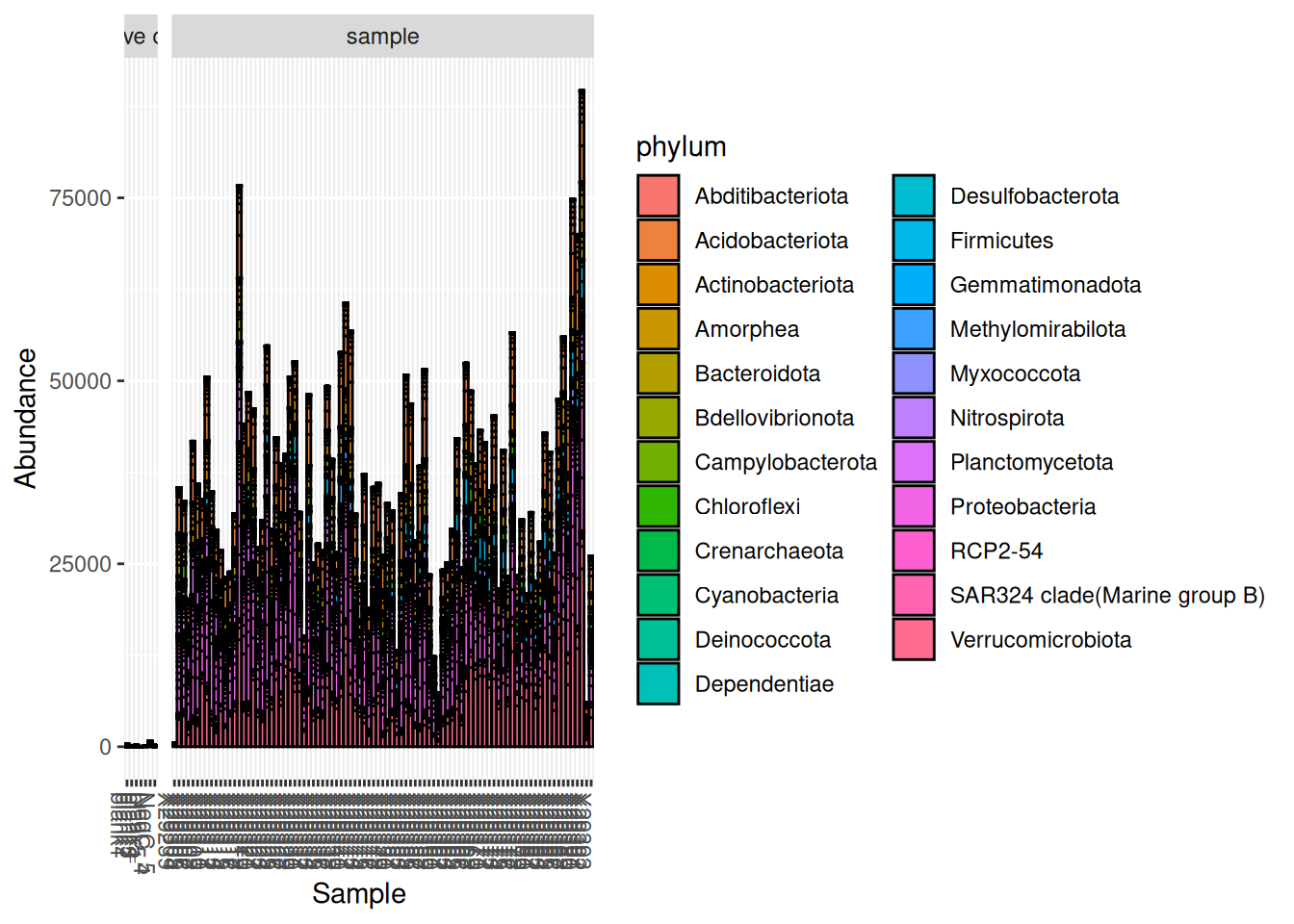

Here we can see that the abundance of these contaminants in the negative controls is very small compared to true samples.

To deal with these OTUs and determine if they are truly contaminants, we can confirm (or infirm) our observations using the package decontam.

R package `decontam`

The R package decontam uses simple statistical tools to identify contaminant automatically^[1]. Visit their webpage for more information.

In this demonstration, we use the function isContaminant with the prevalence method to find which OTUs are contaminants.

# First, add a TRUE/FALSE column "is.neg" to the sample_data
# to identify negative controls
sample_data(otu_table_raw.noPos)$is.neg <-
  sample_data(otu_table_raw.noPos)$sample_type == "negative control"

# Then use the function isContaminant with the default threshold = 0.1
contam.prev <- isContaminant(otu_table_raw.noPos, method="prevalence",
                             neg="is.neg", threshold = 0.1)

table(contam.prev$contaminant)


FALSE  TRUE 
25440    21

The method found 21 contaminant sequences at a threshold of 0.1 (default). In comparison, we had previously identified 302 OTUs present in the negative controls.

Increase the threshold to try and find more contaminants. This more aggressive threshold will identify as contaminants all sequences that are are more prevalent in negative controls than in true samples.

# Use the function isContaminant with the more aggressive threshold = 0.5
contam.prev <- isContaminant(otu_table_raw.noPos, method="prevalence",
                             neg="is.neg", threshold = 0.5)

table(contam.prev$contaminant)


FALSE  TRUE 
25390    71

The method found 71 contaminant sequences at threshold = 0.5.

Inspect contaminants

Visualize the prevalence of these potential contaminants in samples and controls using the presence-absence table created earlier.

# Add a TRUE/FALSE "contaminant" column to identify contaminants
otu_table.pa <- mutate(otu_table.pa, contaminant = contam.prev$contaminant)

# Plot the prevalence of OTU in negative controls vs true samples
ggplot(data=otu_table.pa, aes(x=pa.neg, y=pa.sam, color=contaminant)) + 
  geom_point() +
  xlab("Prevalence (Negative Controls)") + ylab("Prevalence (True Samples)")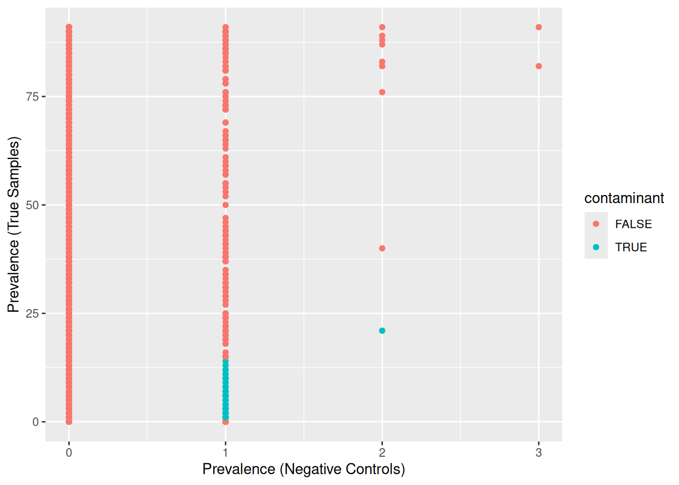

The method identified OTUs that were mostly present in negative controls and few true samples.

# Filter OTU table to keep only OTUs suspected of being contaminants
contaminants <- filter(contam.prev, contaminant == TRUE) %>% rownames()
otu_table_contam <- prune_taxa(contaminants, otu_table_rel)

# Visualize the abundance of these OTUs in all samples
plot_bar(otu_table_contam, fill = "OTU") +
  facet_grid(~sample_type, scales = "free", space = "free") +
  theme(legend.position = "none")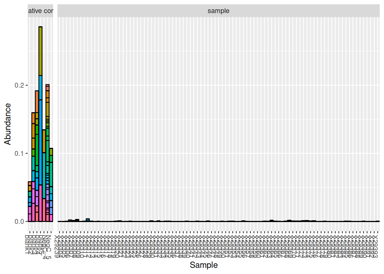

After inspection of these OTUs, it is safe to consider them as contaminants and remove them from the data set. Indeed, their very low abundance suggests that these OTUs may be artifacts or true contaminants from the method. The other OTUs present in the negative controls were most likely coming from true samples and are therefore not considered contaminants. When in doubt, it is best to investigate these OTUs further (look into the taxonomy) to determine if they are truly contaminants.

Clean and save OTU table

remove_taxa

Homemade function remove_taxa: a simplified way of removing a selection of OTU from a phyloseq object.

remove_taxa <- function(badTaxa, physeq){
  allTaxa <- taxa_names(physeq)
  cleanTaxa <- allTaxa[!(allTaxa %in% badTaxa)]
  return(prune_taxa(cleanTaxa, physeq))
}

# Remove samples with low sequencing depth (sampleID = X29239)
otu_table_raw <- prune_samples(
  sample_names(otu_table_raw) != "X29239", otu_table_raw)

# Remove contaminants (note that remove_taxa is a homemade function)
otu_ctrl_clean <- remove_taxa(contaminants, otu_table_raw)

# Remove all controls
otu_ctrl_clean <- prune_samples(
  sample_data(otu_ctrl_clean)$sample_type != "positive control", otu_ctrl_clean)

otu_ctrl_clean <- prune_samples(
  sample_data(otu_ctrl_clean)$sample_type != "negative control", otu_ctrl_clean)

# Save cleaned OTU table
save(otu_ctrl_clean, file = "RData/16S/otu_ctrl_clean.RData")

References

1. Davis, N. M., Proctor, D. M., Holmes, S. P., Relman, D. A., & Callahan, B. J. (2018). Simple statistical identification and removal of contaminant sequences in marker-gene and metagenomics data. Microbiome, 6(1). https://doi.org/10.1186/s40168-018-0605-2

2. Nguyen, N. H., Smith, D., Peay, K., & Kennedy, P. (2014). Parsing ecological signal from noise in next generation amplicon sequencing. New Phytologist, 205(4), 1389–1393. https://doi.org/10.1111/nph.12923